Appendix 10: NZIER CGE Model Specification

The TCDC area model in fact has two key components: a TCDC area social accounting matrix (SAM), and the CGE model itself. The TCDC SAM was derived using the 1996 national input-output tables published by Statistics New Zealand in August 2001, and relevant regional statistics, notable population census and business demographic data. More information about the construction of the TCDC SAM can be obtained from the authors.

The remainder of this section discusses the structure of the CGE model used in the analysis of the indirect impacts of the weather bomb. Again, more details are available from the authors.

In this section we present a description of the used to conduct the quantitative analysis. The model is a 'standard' computable general equilibrium (CGE) model along the lines of de Melo and Tarr (1992), Karadag and Westaway (1999), and Rutherford and Paltsev (1999). [De Melo, Jaime and David Tarr. General equilibrium analysis of U.S. foreign trade policy. Cambridge, MA: MIT Press, 1992.] [Karadag, Metin and Tony Westaway. "A SAM-based computable general equilibrium model of the Turkish economy".Economic Research Paper no. 99/18, Department of Economics, Loughborough University, Leicester, U.K.] [Rutherford, Tom and Sergey Paltsev. "From an input-output model to a general equilibrium model: assessing the excess burden of indirect taxes in Russia". University of Colorado (available at http://debreu.colorado.edu/papers/exburden.html).] These models, and many others like them, can trace their roots to the formalisation by Arrow and Debreu (1954) of the Walrasian general economic structure. [Arrow. K.J. and G. Debreu. "Existence of an equilibrium for a competitive economy",Econometrica22(1954):265-90.]

The main reason for using a CGE model is to provide a quantitative evaluation of economic 'shocks', where such a shock might be a change in government policy, an overseas stimulus (such as an exogenous change in commodity prices) or a natural hazard event. Economic theory, and a good dose of common sense, provides guidelines for judging the impacts of such a shock. However, it is not possible to produce quantitative results from such a qualitative analysis. The principal advantage of using a general equilibrium model, rather than a partial equilibrium (single sector or market) model, is that it enables interactions throughout the economy to be taken account of in a consistent manner.

CGE models are inherently technical, and this poses a challenge in describing them. While we wish this description to be of assistance to technical analysts, we also hope that the non-technical audience will find it useful. Hence, we augment the algebraic presentation of each component of the model with diagrammatic depictions and a written description. Our intention is that one way or another we can convey enough of the flavour of the model so that the results we have generated can be placed in an appropriate context.

As with any economic model, a CGE model is an abstraction that is complex enough to capture the essential features of an economic setting, yet simple enough to be tractable. Our model characterises a small regional economy - Thames-Coromandel District - and comprises four key sectors: consumers, producers, the government and the rest of the world.

Just like in the real world, consumers in our model purchase goods from producers, and in return, they supply the factors of production. The sale of their labour and the 'renting out' of their capital (including land) forms the major source of household income. Consumers, whom we frequently refer to as households, also pay taxes to the government. Final demand by private households arises from nested constant elasticity of substitution (CES) utility functions, i.e. households are assumed to demand goods and services such that they maximise utility subject to a budget constraint. This allows consumer decision making to occur in the form of multi-stage budgeting. At the top level of the household decision, consumers decide which goods and services to purchase from the total pool of products available. At the second level, the consumer decides how much to spend on domestic and imported varieties of each good.

Firms produce goods using primary factors and intermediate inputs. Primary factors in our model include land, labour, and capital. Intermediate inputs can be purchased locally or from imported sources. Production activities are assumed to exhibit constant returns to scale and individual firms behave competitively, selecting a level of output such that marginal cost at that output level equals the given market price. Output is differentiated between goods destined for domestic and export markets.

Government expenditures and investment demand are exogenous. Funding of government expenditures is provided by various tax revenues and import tariffs. Real government expenditure is held constant under all counter-factual scenarios via lump sum transfers to households. Hence, the effect of such transfers is neutral. Because private consumption equals the income from primary factors plus net transfers to the consumer by the government, Walras law is satisfied.

In the TCDC context, the rest of the world encompasses everything outside of the TCDC area. Thus, the TCDC economy imports from and exports to other New Zealand district council areas. However, in the model the TCDC economy is treated as if it were effectively borderless, such that no barriers to trade exist between TCDC and the rest of New Zealand, and that no rate of exchange exists to equilibrate prices between TCDC and other regions.

The model includes an explicit treatment of unemployed labour: unemployed labour is available for hire, subject to the constraint of 'downward sticky' wages; that is, the real wage is prohibited from falling. This has the practical consequence that the unemployed will be encouraged into the workforce before the price of labour is bid up.

A CGE model works by using data to describe the economy in a benchmark year, and by specifying hundreds of mathematical equations to represent the relationships between all such data values. By then varying one or more elements so as to 'shock' the economy, we can trace throughout the economy the changes in the values of the data items. We say the model is 'calibrated' when it is specified and configured in such a way that a solution to the mathematical system replicates the benchmark data. Choosing the appropriate elements to shock is the process by which a policy simulation is undertaken.

The mechanism by which the model derives a new solution, following a shock, is to find the set of prices that clears all markets. For example, the price of all goods in the economy change so that all goods markets are cleared. Market clearing simply means that supply equals demand.

For this study, we have aggregated the data base to reflect 9 production sectors and commodities. These are: agriculture and other primary production; manufacturing; utilities and construction; retail and wholesale trade; finance, insurance and business services; owner-occupied dwellings; government administration; health, education and other personal services; and, other services.

As noted above, the basis for the CGE analysis contained in this report is a social accounting matrix (SAM) for the TCDC economy, which in turn has been constructed using the Inter-Industry Study 1996, the New Zealand Institutional Sector Accounts Experimental Series 1987 - 1998 and a range of regional statistics, all published by Statistics New Zealand.

n this section we present a more detailed description of the model. The model is coded using the GAMS/MPSGE software. [Rutherford, T.F. (1999). "Applied general equilibrium modelling with MPSGE as a GAMS subsystem: An overview of the modelling framework and syntax",Computational Economics; and www.gams.com.] Accordingly, just three sets of 'central variables' are required to formulate the model:

• vector of non-negative commodity prices, including one for each good (intermediate and final) and primary factor of production;
• non-negative vector of activity levels representing production activities; and
• vector of income levels, one for each household and government entity in the model.

An equilibrium in these variables must satisfy a system of three classes of nonlinear inequalities: zero-profit conditions, market clearance conditions, and income balance equations. While the MPSGE software allows the model to be formulated in a compact manner, it is not particularly revealing to the uninitiated. Hence we do not present the code here. [The MPSGE code and a complete technical description of the model can be requested from the authors.]

10.3.1 Production

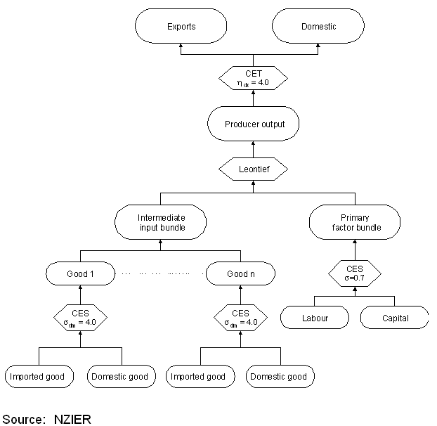
Production sectors are assumed to (potentially) produce two types of commodities: domestic goods D_i and goods for export X_i. These two goods are assumed to be imperfect substitutes, and have a constant elasticity of transformation. In the production process, each sector uses capital, labour, and intermediate goods. As such, the ith sector's production function can be given by:

(1)

where g is the output transformation function and f is the input transformation function. As previously noted, output transformation is assumed to be via the constant elasticity of transformation (CET) function, which can be written:

(2)

where  and are the benchmark levels of output destined for the domestic and export markets, respectively, and  is the benchmark value share of domestic sales in total output for sector i. The elasticity of transformation is given by .

The input combination function is a combination of two aggregator functions, and for sector i can be specified as follows:

(3)

where LF is a 'Leontief' aggregate and CES denotes a constant elasticity of substitution aggregate. A Leontief production function implies an elasticity of substitution equal to zero, and is a special case of the more general CES family of functions. We can state equation (3) algebraically according to the following expression:

(4)

where A_ji denotes the quantity of intermediate input from sector j required to produce a unit of output in sector i, and a_ji represents the fixed input-output coefficients.

The CES aggregation of capital and labour can be written algebraically as:

 (5)

where  and are, respectively, the benchmark levels of capital and labour used in sector i, δ_i is the share parameter of capital and labour, respectively, and the elasticity of substitution between capital and labour is given by ; for all sectors this elasticity has a value of 0.7. [The value of capital-labour elasticities of substitution (in fact, as with all elasticity values) is subject to much debate, and there exists little empirical work specific to the New Zealand economy to support particular values. The elasticity of substitution values assumed in this study are based on a wide review of the substitution elasticity literature.]

Finally, we come to the algebraic representation of intermediate goods, A_ji. As depicted in equation (3), the input transformation function combines intermediate goods with a composite 'value added' good, i.e. the value-added composite good refers to the combination of capital and labour. But the intermediate goods, A_ji, are themselves an aggregation of domestically produced and imported goods. We use A_ji, where the A stands for 'Armington', to represent the intermediate goods. [Armington, P.A. (1969). "A theory of demand for products distinguished by place of production".IMF Staff Paper16(1):159-178.] The Armington aggregation of domestic and imported varieties of a good may be stated algebraically as:

 (6)

where ZD and ZM denote, respectively, the domestic and imported varieties of the intermediate good, Z, used in sector i. The elasticity of substitution between domestically available and imported goods is denoted and is equal to .

The structure of the production function is illustrated in Figure 1.

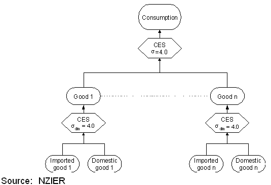
For this study the model is configured with a single 'representative agent'. In essence, this means that the all households in the economy are assumed to behave identically. Households are assumed to maximise utility subject to a budget or income constraint. We aggregate all of the consumption goods in a manner analogous to the preceding production activities. The household then 'consumes' the aggregate consumption good, which can be thought of as a consumer price index (CPI) basket of goods. The 'production' of the CPI good is shown in Figure 2.

In the same way that intermediate goods enter the production function as an Armington aggregate of imported and domestically produced goods, all goods entering the consumption activity are also combined in line with the Armington assumption.

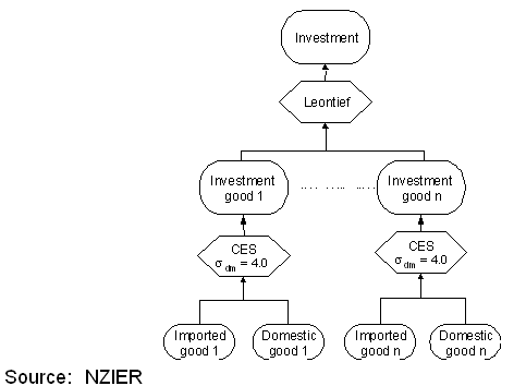
Even though the model is static, it is necessary to account for the investment and savings that take place during the period of analysis. Generally speaking it is assumed that the capital stock is fixed, as is standard practice in a comparative static analysis. Hence, investment does not add to the current capital stock, but for accounting purposes, we need to specify the size and composition of the investment demand.

The model does not distinguish between public and private investment. Instead, fixed and inventory investment is combined into a single set of sectoral investment accounts. The aggregate level of investment is determined by the available supply of savings in the economy, where the latter is the sum of private, public and foreign savings, plus depreciation.

Investment demand is depicted in Figure 3. The interpretation is self evident following that for production and household consumption.

Finally, we have a government sector. The government in our model purchases a range of goods on behalf of households, for example, education and health services. The structure of government demand is conceptually identical to investment demand. Of course, the value shares of goods entering the demand activity are not the same as for investment, and like all other value shares, are determined from the benchmark data.